CorefieldBiophysics
Bioelectromagnetic simulation studies

Every exposure result, with its error bars attached.

Corefield Biophysics runs simulation studies for medical devices, MRI hardware and wireless products. We compute SAR, absorbed power density, induced fields and tissue heating, in-house with our own solver, EMVIE.

  • MRI implant safety
  • SAR compliance
  • Power density above 6 GHz
  • EU Directive 2013/35/EU
  • Neurostimulation
  • Cell-scale stimulation
  • Second opinions
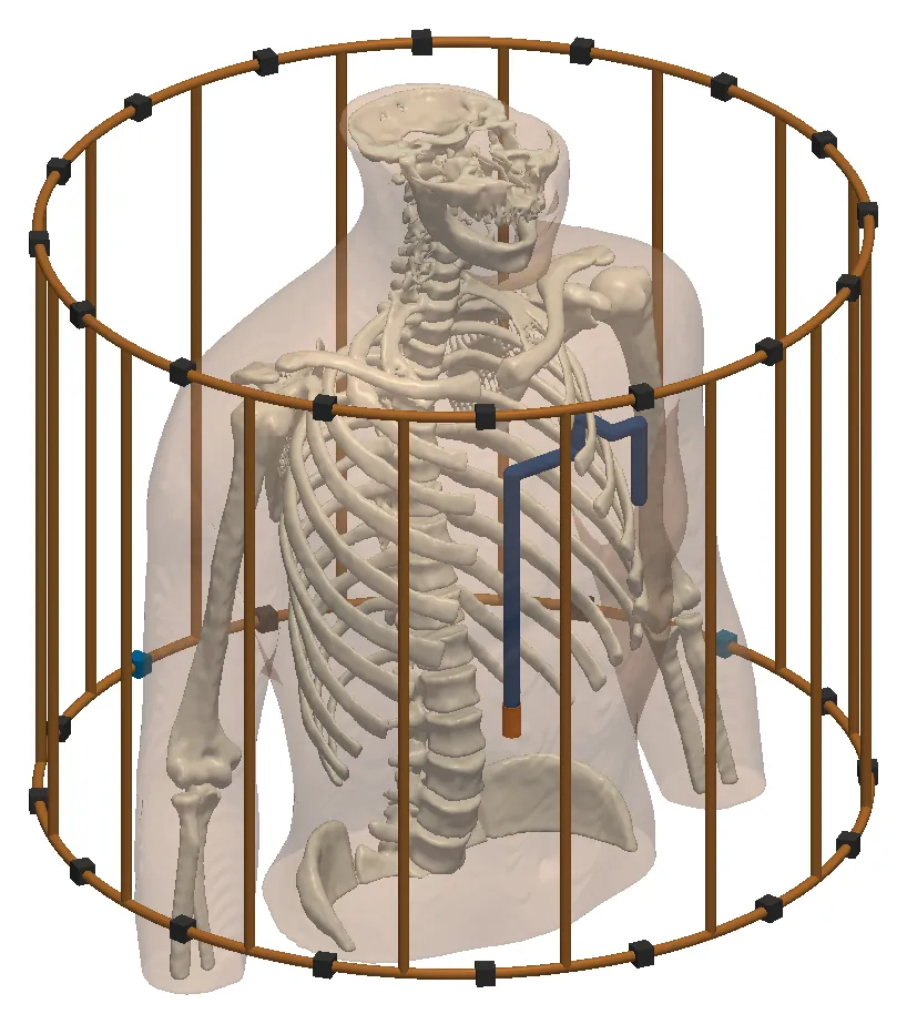
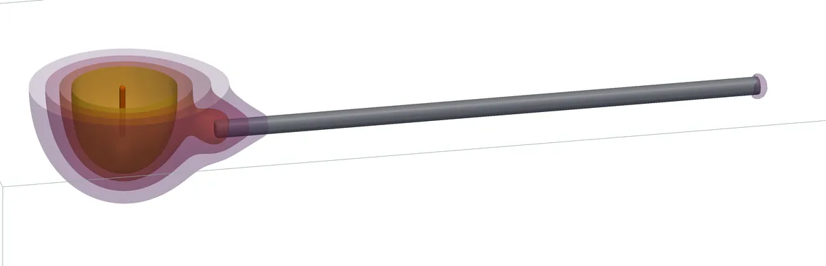
Translucent human trunk with its skeleton inside a cylindrical 16-rung birdcage coil, with an implanted lead routed over the ribs to its electrode tip BodyParts3D © DBCLS, CC BY 4.0
MRI implant safety · 3 T, 128 MHz

An implanted lead in the trunk inside a 16-rung birdcage coil. At B1 = 2 µT, peak SAR over 1 g at the tip is 4.42 W/kg, against 2.07 W/kg without the lead.

0.3%agreement between our two independent solvers on a matched 8-channel 7 T dipole array
20head models in our population study of parallel-transmit safety margins
6of 6standard validation dipoles within the ±10 % system-check tolerance, under both SAR averaging rules
DC–300GHzfrom brain stimulation to millimetre-wave skin exposure
Services

Six studies, each with a stated deliverable

We run every study in-house with our own solver, EMVIE. You receive the results, a report and the inputs behind each number.

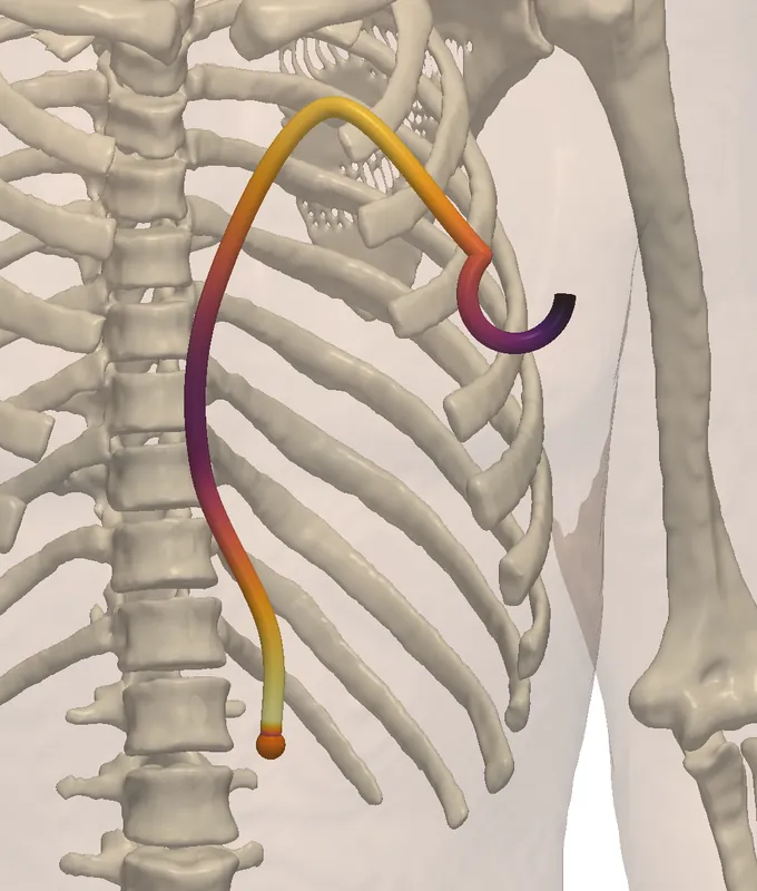
Trunk with skeleton and an implant lead route drawn as a tube coloured by the tangential incident electric field along itBodyParts3D, CC BY 4.0
ISO/TS 10974 · Tier 3

MRI RF safety of active implants

Tip heating of your lead for each route and body position, at 1.5 T and 3 T.

Read moreShow less

We compute the transfer function of your lead and the incident fields along clinical lead routes in the body, at 1.5 T and 3 T. Together they give the tip heating for each route and body position.

Also offered: local-SAR safety margins for 7 T parallel-transmit head arrays, with Q-matrices and virtual observation points.

You receive
Lead transfer function, incident-field library, tip SAR and temperature rise per route, and the validity limits of the lead model
Standard
ISO/TS 10974, Tier 3
Turnaround
On request
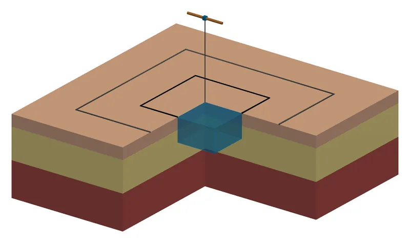
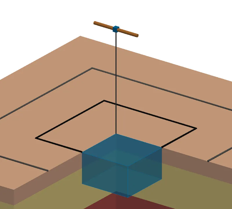
Close-up of a half-wave dipole above layered tissue, its feed line dropping to the averaging cube marked at the surface
IEC/IEEE 62704-1 · 62209-1528

SAR and psSAR near the body

Peak spatial-average SAR over 1 g and 10 g for devices used against the head or body.

Read moreShow less

Peak spatial-average SAR over 1 g and 10 g for devices used against the head or body. Before we model your device, we check the set-up on the standard validation dipoles, as a SAR laboratory does in its system check.

You receive
psSAR over 1 g and 10 g per configuration, SAR maps, a grid convergence check and the consensus-dipole check in the same report
Standard
IEC/IEEE 62704-1; system check against the IEC/IEEE 62209-1528 targets
Turnaround
On request
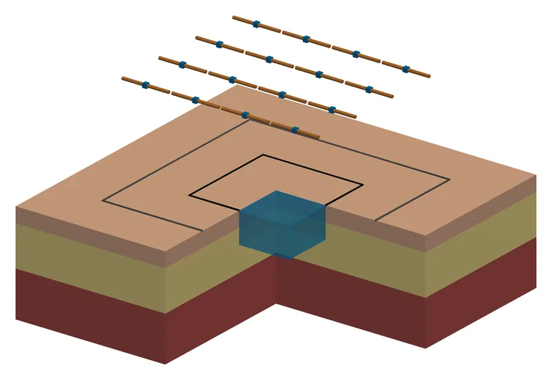
Four by four dipole array above a cut-away block of skin, fat and muscle, with two square averaging areas marked on the skin
IEC/IEEE 63195 · ICNIRP 2020

Power density above 6 GHz

Absorbed power density over 1 cm² and 4 cm² and the skin temperature rise for 5G and millimetre-wave devices.

Read moreShow less

Absorbed power density over 1 cm² and 4 cm² and the skin temperature rise for 5G and millimetre-wave devices. We state how much the result changes with the skin model and the averaging definition.

Pictured: a 4 × 4 dipole array at 30 GHz over skin, fat and muscle, with the 1 cm² and 4 cm² averaging areas on the skin.

You receive
Peak absorbed power density over 1 cm² and 4 cm², maps on the skin, the temperature rise and its spread over skin models
Standard
IEC/IEEE 63195; limits of ICNIRP 2020 and IEEE C95.1-2019
Turnaround
On request
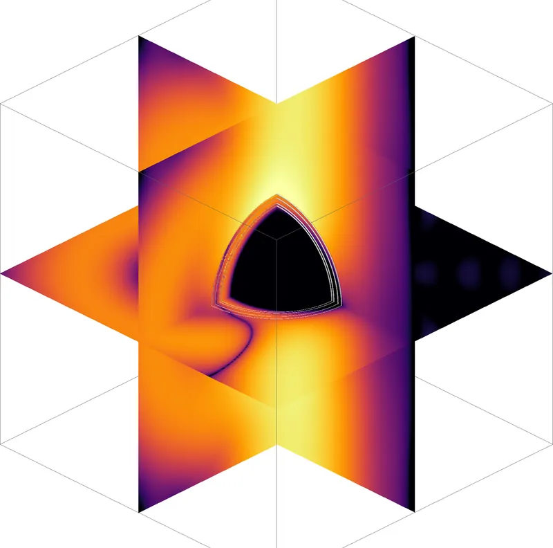
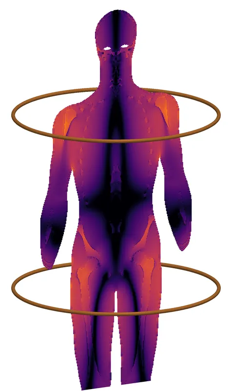
Human body between the two loops of an MRI gradient coil, coloured from dark purple to orange by the induced electric fieldBodyParts3D, CC BY 4.0
Directive 2013/35/EU · ICNIRP 2010

Low-frequency exposure at work

Electric fields induced in the body by coils and other low-frequency sources, including MRI gradients.

Read moreShow less

Electric fields induced in the body by coils and other low-frequency sources, including MRI gradients. For pulsed and non-sinusoidal waveforms we apply the weighted peak method, in the frequency domain and in the time domain.

Pictured: a body between the loops of a gradient coil; the solver computes the induced field in nerves and muscle.

You receive
Exposure index per tissue against the exposure limit values, the 99th percentile over 2 mm cubes, and the weighting filter used, stated with each result
Standard
Directive 2013/35/EU, Annex II; ICNIRP 2010
Turnaround
On request
pair 1 · f₁pair 2 · f₂
TI · tES · TMS

Neurostimulation field planning

Electric fields in the brain for temporal-interference, transcranial current and magnetic stimulation.

Read moreShow less

Electric fields in the brain for temporal-interference, transcranial current and magnetic stimulation. We compare electrode montages and currents for your target. We also show how much the target field depends on each tissue's conductivity.

You receive
Field maps in the target and outside it, a montage and current proposal, and the sensitivity of the target field to each tissue
Standard
No product standard applies; methods and uncertainty are reported in full
Turnaround
On request
YOUR STUDYEMVIE RECOMPUTATIONCOMPARISON ranked by effect
Any of the standards above

Independent second opinion

We rebuild the key cases of another team's study with our own solver and explain every difference.

Read moreShow less

You send us a simulation report or the simulation files from another team or tool. We rebuild the key cases with our own solver and explain every difference we find.

You receive
A written review, an independent recomputation of the key numbers, and the issues ranked by their effect on the result
Standard
The standard the original study follows
Turnaround
On request

We offer fixed-price studies, ongoing support during development, and independent reviews. Turnaround depends on the model and the number of cases, so we state it in each proposal.

Capabilities

One verified engine, from quasi-static to millimetre wave

We wrote the solvers we use, and we run them only in-house, for our clients' studies. Every change runs through an automated test suite, and results are bit-identical for any number of CPU threads.

Volume integral equationFinite-difference time domainTransmit arrays and coilsLeads and transfer functionsQuasi-static fieldsBioheat and damageTwo averaging rules from one solveWeighted peak methodAdjoint sensitivitiesCell-scale stimulationHierarchical matrices (H-LU)Head-to-cell coupling
Read more: what each capability coversHide the details
RF

Volume integral equation

GPU-accelerated, octree meshes, and a dispersion correction that removes the bulk part of the grid error at gigahertz frequencies.

RF

Finite-difference time domain

GPU solver with dispersive tissues, thin wires, lumped ports and absorbed power density readouts.

MRI

Transmit arrays and coils

Ported dipole arrays, matching networks, RF shields, birdcages, Q-matrices and virtual observation points.

Implants

Leads and transfer functions

Insulated leads in tissue, reciprocity transfer functions and stored incident-field libraries for Tier 3.

Low frequency

Quasi-static fields

Multigrid electro- and magneto-quasi-static solvers, contact electrodes, anisotropic tissue and field-dependent conductivity.

Thermal

Bioheat and damage

Pennes bioheat with perfusion, pulse trains, blood cooling, vaporisation and Arrhenius tissue damage.

SAR

Two averaging rules from one solve

Cube-averaged SAR over 1 g and 10 g under the IEC/IEEE 62704-1 rule, which allows up to 10 % air in a cube, and under a stricter rule with no air, from the same field.

New · Low frequency

Weighted peak method

Exposure index for pulsed and non-sinusoidal fields against the ICNIRP 2010 limits and the exposure limit values of Directive 2013/35/EU, in the frequency and the time domain.

New · Neurostimulation

Adjoint sensitivities

The gradient of a target-field objective with respect to every tissue conductivity and every electrode current, for about the cost of two field solves. It covers single-pair and temporal-interference stimulation.

New · Cells

Cell-scale stimulation

The membrane response of neurons and other cells in stimulation fields, with the cell, the surrounding fluid and the electrodes coupled in one bidomain boundary-element model. Verified at second order against exact solutions; it reproduces the published bidomain BEM cases. In final testing. More

New · Fast algorithms

Hierarchical matrices (H-LU)

Compressed boundary-element matrices: low-rank far-field blocks by adaptive cross approximation and a factorization in compressed form. 320 000 unknowns factor in 16.7 GB, where the dense matrix would take 819 GB. More

New · Cells

Head-to-cell coupling

The cell model takes its incident field from our own head solution, for example under a TMS coil, instead of a uniform field.

New in the solver · cell scale

Cell-scale stimulation with a bidomain boundary-element solver

How the membrane of a neuron responds to TMS, deep-brain, temporal-interference and electrode fields. The cell, the fluid around it and the electrodes are solved together, so the cell changes the field and the field changes the membrane voltage. The method builds on the bidomain BEM of Czerwonky, Aberra and Gomez (J. Neural Eng., 2024) and Hasan et al. (IEEE J-ERM, 2026). We reproduce their published cases and extend the method in the five ways below.

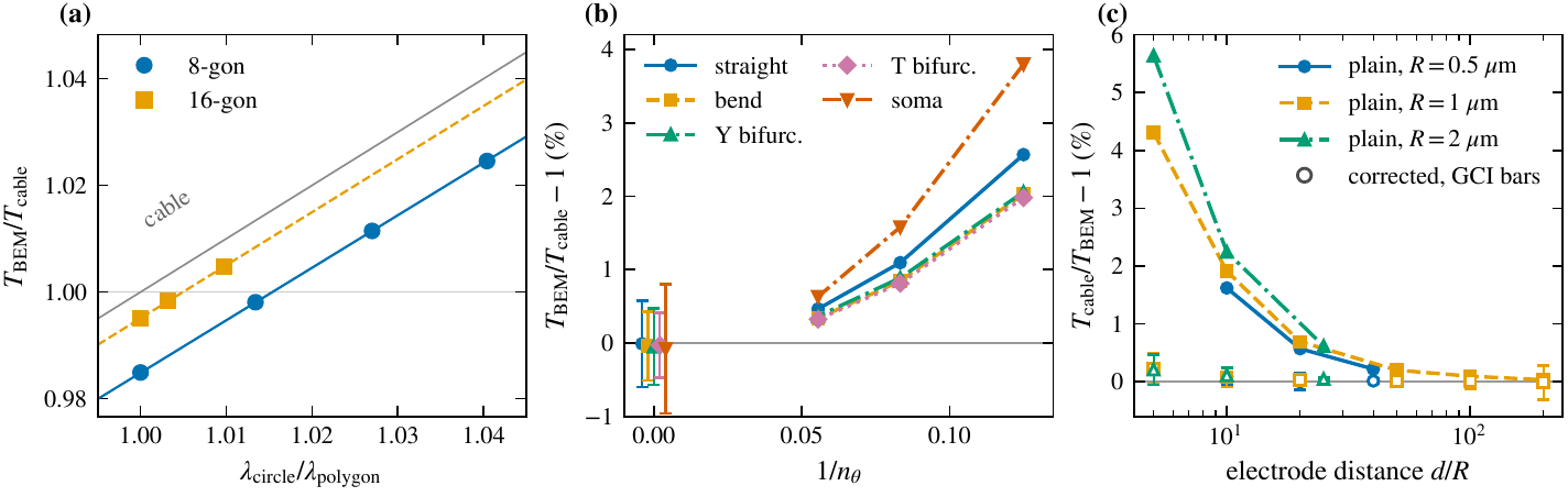
Three plots comparing bidomain BEM and cable-model thresholds of Hodgkin-Huxley axons. (a) Ratio of BEM to cable threshold for 8-gon and 16-gon cross-sections, approaching the cable line as the polygon is refined. (b) Threshold gap for a straight axon, a bend, Y and T branch points and a soma, falling to zero within the error bars as the mesh is refined. (c) Cable threshold above the BEM threshold by up to about 5.6 percent for a point electrode within 5 to 20 fibre radii, and near zero for the corrected cable.
When is the classic cable model right? (a) On a straight axon, the gap between BEM and cable thresholds comes from the polygonal cross-section of the mesh and closes as the polygon is refined. (b) Bends, branch points and the soma agree with the cable within the numerical uncertainty. (c) Near a point electrode the cable model overestimates the threshold, by up to 5.6 % within 5 to 20 fibre radii; our corrected cable (open markers) reproduces the full model to 0.23 % or better down to five radii.

What our solver adds to the published bidomain BEM

Each item is a result of our own runs. The methods paper is in preparation.

Reproduced first

The published cases

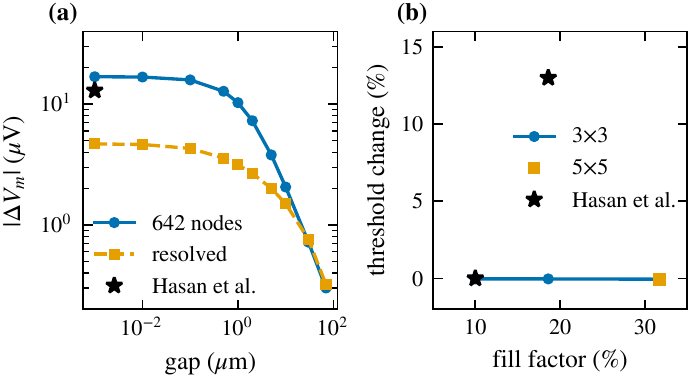
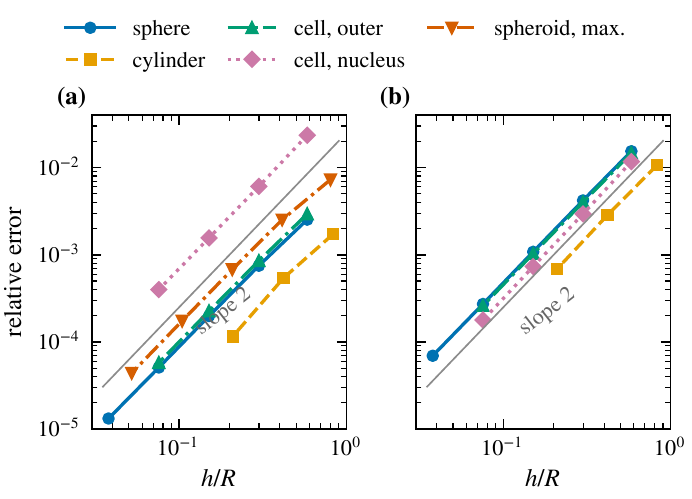
The synthetic axon cases of Hasan et al. (two axons and a multi-axon block) are reproduced on meshes of the same size. One result differs: we find no rise of the threshold with packing density in their Fig. 15. Exact solutions for a sphere, a cylinder, a cell with a nucleus and a prolate spheroid converge at second order, and an independent finite-volume solution agrees to 0.005 % or better.

Speed and memory

H-matrix algebra for large cells

Blocks between distant parts of the cell are stored in compressed form. A cell model with 159 058 nodes runs in 12.0 GB of matrices, where a dense solver would need 0.8 TB. Details below.

Robustness

A charge constraint

A closed membrane carries no net charge. The solver enforces this exactly, with one extra row per membrane. That removes the one poorly conditioned mode of the system at low membrane conductance, and leaves the thresholds unchanged.

Realistic neurons

A reconstructed layer 2/3 pyramidal cell

Meshed with 18 635 to 74 659 nodes and compared with a NEURON cable model of the same tree, both with the Hodgkin-Huxley membrane. The 2 to 3.5 % gap reported in the literature appears only on the coarse mesh. Once the mesh converges, the BEM threshold lies 0.7 to 0.8 % below the cable for a field along the apical axis and for a point source, and 2.7 % below it for a transverse field.

In review

Blue Brain ion channels in the membrane

The cell's own channel set (11 channels and the calcium pool of the L2/3 cell) now runs inside the BEM membrane. On a membrane patch, the spike times match NEURON 9.0.2 to within 0.07 to 8.5 µs over five spikes in 40 ms.

Multiscale

Coupling to head models

The cell can take its field from our own head solution instead of a uniform field. In a first test with a figure-8 TMS coil, the local head field changed the threshold of an axon by 0.7 to 8.5 %, with either sign, at six cortical sites.

Two plots. (a) Peak membrane polarization of a passive axon against the gap to a firing neighbour, for the 642-node mesh and a resolved mesh, with the published value as a star near the 642-node curve. (b) Threshold change of the central axon against the volume fill factor for 3 by 3 and 5 by 5 blocks, flat at zero, with the published 13 percent rise as a star.
Reproducing Hasan et al. (a) Polarization of a passive axon by a firing neighbour against the gap between them, on their 642-node mesh and on a resolved mesh. (b) Threshold of the central axon of a block against the fill factor. Stars: values read from Hasan et al., IEEE J-ERM 2026.
Two log-log plots of the relative error of the membrane voltage against the mean edge length for a sphere, a cylinder, a cell with a nucleus and a prolate spheroid; all lines follow slope 2, in the steady state and at one time constant.
Verification against exact solutions. The error of the membrane voltage falls with the square of the triangle size for every cell shape. (a) Steady state. (b) At one membrane time constant.
New in the solver · fast algorithms

Hierarchical-matrix (H-matrix) acceleration

In a boundary-element model every surface node interacts with every other, so the matrix is dense: memory grows with the square of the node count. Interactions between groups of nodes that are far apart compared with their size are smooth, and a few terms describe them. An H-matrix stores those blocks in this compressed, low-rank form, built by adaptive cross approximation, and keeps only the near field in full. The whole matrix is then factored in compressed form (H-LU).

near field stored in full far field column × row, rank of tens Blocks grow with the distance from the diagonal.
The block partition. Nodes are sorted into a tree of nearby groups. Blocks between neighbouring groups stay dense; blocks between distant groups are stored as a thin column times a thin row. Schematic, drawn for this site.
16.7GB

320 000 unknowns factored in 2.0 h. The dense matrix alone would take 819 GB.

30–58

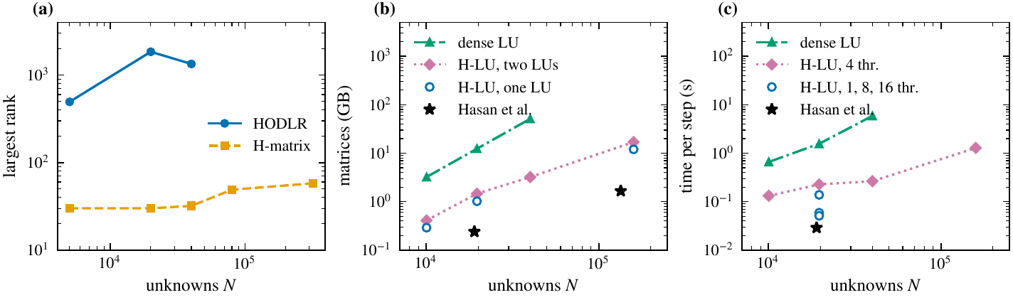
Largest block rank after the factorization, bounded from 5 000 to 320 000 unknowns. A HODLR matrix, the format of the earlier cell solver, reaches rank 1 848 at 20 000 unknowns on the same points.

1.04–1.17×

Peak memory of the factorization over its data, because every update is written into existing blocks. The published recursive HODLR setup peaked at about 200 times its compressed matrices: 332.78 GB for 1.66 GB, eight neurons.

2 × 10⁻⁹

Largest difference from the dense solution, relative to the amplitude, on the exact-solution cases at a block tolerance of 10⁻⁶: four orders of magnitude below the discretization error.

Three log-log plots against the number of unknowns. (a) Largest block rank: HODLR rises to about 1 850, the H-matrix stays between 30 and 58. (b) Memory of the matrices: dense LU rises to about 50 GB at 40 000 unknowns, H-LU stays one to two orders lower up to 159 058 unknowns, with the published values as stars. (c) Time per step: dense LU is slowest; H-LU with 1 to 16 threads approaches the published value.
Measured cost. (a) Largest block rank on bath-and-axon point sets. (b) Memory kept and (c) time per step for a soma with axons; stars: values reported by Hasan et al. for one and eight neurons. A cell model with 19 658 nodes keeps 1.02 GB of matrices against 12.37 GB dense. The gains are memory, setup time and bounded ranks; we do not claim a faster time step than the published HODLR solver.
Verification

Checked twice, by different methods

We test against exact solutions and published benchmarks, and compute key results with two independent solvers. The record below comes from our own runs.

How close each check comes to its reference

Relative difference, log scale. Further left is closer agreement.

second solverexact or resolved referencefinite differences, publication, grid
1, 4 and 8 CPU threads: bit-identicalSAR ratios of a published 7 T design: within 0.03IEC/IEEE 62704-1 system check: +4.5 % and +9.6 % of ±10 %
2.1–2.5×less power

Across the 6 GHz boundary. A device that just passes below 6 GHz may emit less than half that power just above it.

Read moreShow less

Above 6 GHz the limit changes from peak SAR over 10 g (2 W/kg) to absorbed power density over 4 cm² (20 W/m²). In 95 runs with dipoles, arrays and patch antennas over three skin models, 5 to 15 mm from the skin and 3 to 24 GHz, the second limit allowed 2.1 to 2.5 times less power than the first would have at the same frequency, whatever the source. So a device that just passes below 6 GHz may emit less than half that power just above it.

Read more: the full verification recordHide the full record
CheckCompared withAgreementStudy
8-channel 7 T dipole array with matching: accepted power, absorbed power, peak 10 g SARSecond solver (FDTD vs integral equation)within 0.3 %7 T safety margins
Insulated implant lead, tip current at 64 and 128 MHzResolved axisymmetric referencewithin 0.5 %Implant heating
Dipole over a flat phantom, IEC/IEEE 62704-1 geometry: peak SAR over 1 g and over 10 gSecond solver, both converged at the surface peak0.1 % and 1.2 %RF dosimetry
30 GHz dipole over skin, peak absorbed power density, a case computed by 11 research groupsSecond solverwithin 0.6 %Millimetre-wave skin
Fractionated dipole of a published 7 T design: SAR ratios (dimensionless)Published design studywithin 0.037 T safety margins
Spheres and layered bodies in a plane wave at 0.9 and 3 GHz: total absorbed power, extrapolated to zero cell sizeExact solutionwithin 1.5 %RF dosimetry
The same bodies: peak SAR over 10 g on the finest gridsSecond solverwithin 2.2 %RF dosimetry
Same case on 1, 4 and 8 CPU threadsRepeated runsbit-identicalAutomated test suite
Code verification to IEC/IEEE 62704-1, and the new methods
CheckCompared withResultStudy
IEC/IEEE 62704-1, clause 8, automated test suite for our FDTD solver
8.2.2 planar dielectric boundary: TM reflection onto a lossy dielectric, grids of 1 and 0.5 mmExact Fresnel coefficientwithin 0.06 %
order 1.9 to 2.1
Extrapolated value; the error falls with the square of the cell size, as expected
8.3.4 system check: dipole over the flat phantom at 3000 MHz, FDTD on a 1 mm grid, peak SAR over 1 g and 10 gTarget of the standard, ±10 %+4.5 % and +9.6 %Inside the tolerance
8.2.1 free-space propagation, 8.3.1 generic dipole, 8.3.2 microstripValues and limits of the standardpass8.2.1 also has our own lossy-tissue extension: 1 of its 6 checks sits at its 2 % limit
8.2.3 open boundaries: reflection of the absorbing boundaryOur own −40 dB limit; the standard's range is not openly publishedpassNot the standard's number
Adjoint gradients of low-frequency field objectives
Gradient with respect to tissue conductivity, electrode voltage and current, on layered models and a 1 mm head with 3.87 million voxelsCentral finite differences of the forward solverwithin 2.4 × 10⁻⁷Relative difference, worst case
Normalised conductivity sensitivity, concentric shellsClosed formwithin 1 % from 1.5 mm
0.006 % at 0.5 mm
Grid refinement
Temporal-interference envelope, two channelsCentral finite differenceswithin 3.1 × 10⁻⁷Relative difference, worst case
Cost of one gradient, 1 mm headOne forward solve1.66 solvesFinite differences would need 2 solves per tissue
Weighted peak method for pulsed low-frequency fields
Sinusoids, two-tone signals, a rectangular pulse train and a damped sinusoidClosed-form exposure indexwithin 5 × 10⁻⁶Relative difference
Trapezoid and double pulse of a published study: ratio of the frequency-domain to the time-domain indexL. Giaccone, Phys. Med. Biol. 68 (2023) 095001, Fig. 4: 0.91 and 1.380.908 and 1.377Agrees to the two decimals published
Time-domain weighting filter, all eight limit sets of ICNIRP 2010 and the DirectiveThe 3 dB and 90° tolerance of the ICNIRP 2010 annexworst 2.85 dB, 70°Inside the tolerance
Absorbed power density above 6 GHz
Plane wave at 6 GHz onto muscle: power entering the surface, grids of 0.5 to 0.0625 mmExact solution+2.1 % to +0.04 %The error falls with the square of the cell size
Dipoles and arrays over skin, 6 to 24 GHz: peak SAR and absorbed power density, 0.25 against 0.125 mm gridsGrid refinementwithin 2.5 %
ratios within 0.4 %
Grid uncertainty of our 95-case sweep

The clause 8 criteria are those of the 2017 edition, as quoted in open sources. The 2026 edition keeps the structure of clause 8. Two items need data the standard does not publish openly, so they are not in the suite: the SAR averaging test with the SAR Star (8.2.4) and the SAM phantom with the generic phone (8.3.3). The feed-point impedance of 8.3.4 is reported but not judged, because the standard does not specify the feed.

The weighted peak method and the adjoint gradients are new in November 2026. Both pass the checks above. They now go through our full test suite before we use them in client studies.

The papers behind these studies are listed under Research once they are submitted.

Verification against measurement

The set-up every SAR laboratory checks itself against

Exact solutions and a second solver show that the equations are solved correctly. The next question is whether the result matches the physical world. Here we compare EMVIE with published measurements and with the reference values that measurement laboratories use, and we say which is which.

Measurement

A quantity measured on a physical set-up, shown with the uncertainty its authors state.

Consensus target

A reference value fixed by an international standard. It was computed and checked by measurement when the standard was written. Every accredited SAR laboratory must reproduce it to within ±10 % in its system check. Matching it shows that EMVIE reproduces the industry's reference set-up; it is not a new measurement.

Case 1 · consensus target

Standard validation dipoles over the flat phantom

On the 2 mm grid, all six dipoles from 835 to 3000 MHz are inside the ±10 % tolerance under both SAR averaging rules.

Tissue-simulating liquid 1 g / 10 g cube Flat phantom shell Half-wave dipole 1 W forward power
The system-check set-up, schematic and not to scale. The SAR peak sits at the inner surface of the phantom, above the feed.
Read moreShow less

These are the half-wave dipoles and the liquid-filled flat phantom of IEC/IEEE 62209-1528 and IEC/IEEE 62704-1, from 835 to 3000 MHz. EMVIE models each dipole as a fed thin-wire antenna, solves it together with the phantom and scales the result to 1 W forward power.

On the 2 mm grid, all six dipoles are inside the ±10 % tolerance under both SAR averaging rules. Peak SAR over 1 g is within −3.9 to +1.4 % of the target. Over 10 g, the IEC/IEEE 62704-1 rule, which allows up to 10 % air in a cube, gives +2.8 to +6.2 %. A stricter rule with no air in the cube gives −2.1 to +0.3 %.

EMVIE peak SAR relative to the standard targets, 2 mm grid

EMVIE ÷ target − 1. Shaded: the ±10 % band a laboratory's system check must meet.

1 g, both rules10 g, up to 10 % air10 g, no air
Read more: values per dipole, the 1 mm grid and our findingsHide the values
2 mm grid, per 1 W forward power
FrequencyPeak SAR, 1 g (W/kg)
EMVIE / target
Deviation10 g, up to 10 % air (W/kg)
EMVIE / target
Deviation10 g, no air (W/kg)
EMVIE / target
DeviationTarget from
835 MHz9.62 / 9.56+0.7 %6.47 / 6.22+4.0 %6.17 / 6.22−0.7 %IEC/IEEE 62209-1528 ¹
900 MHz10.99 / 11.0−0.1 %7.27 / 7.07+2.8 %6.92 / 7.07−2.1 %IEC/IEEE 62704-1
1800 MHz38.5 / 38.4+0.3 %20.8 / 20.1+3.6 %19.7 / 20.1−1.9 %IEC/IEEE 62209-1528 ¹
1900 MHz40.1 / 39.7+1.0 %21.5 / 20.5+4.8 %20.4 / 20.5−0.6 %IEC/IEEE 62209-1528 ¹
2450 MHz53.1 / 52.4+1.4 %25.5 / 24.0+6.2 %24.1 / 24.0+0.3 %IEC/IEEE 62209-1528 ¹
3000 MHz62.9 / 65.4−3.9 %26.7 / 25.3+5.4 %25.0 / 25.3−1.2 %IEC/IEEE 62704-1
1 mm grid, per 1 W forward power
Frequency1 g, up to 10 % air10 g, up to 10 % air1 g, no air10 g, no airStatus
900 MHz+1.5 %+2.4 %not runnot runInside the tolerance
1900 MHz+4.1 %+5.3 %rerun pendingrerun pendingInside the tolerance; the no-air values of the first run had a round-off error, since fixed
3000 MHz+1.3 %+6.8 %−0.2 %+4.4 %Inside the tolerance; no-air cubes slid to the surface. Not yet grid-converged: the values still rise from 2 to 1 mm, and the 0.5 mm run decides

¹ Values of the standard's target table as quoted in public reference-dipole calibration reports. The 2450 MHz targets are not yet confirmed in a source we have opened. We are checking them, and the dipole lengths at 1800 to 2450 MHz, against the published standard. The lengths we use are within 0.5 mm of commercial validation dipoles.

Resolved finding. On the 1 mm grid at 3000 MHz the no-air rule first read 8.0 % low on 1 g and 6.6 % low on 10 g. The cause was where the cubes sit: a cube centred on a voxel and grown in whole layers stops up to 0.7 mm short of the surface. With the cubes slid continuously until their face touches the surface, the 1 mm values are −0.2 % on 1 g and +4.4 % on 10 g, both inside the ±10 % tolerance. The 2 mm grid has fewer than 10 cells per wavelength in the liquid at 3000 MHz, so its 1 g shortfall is mostly grid resolution.

Phantom size. A larger phantom at 1900 MHz changes peak SAR by less than 0.1 %.

Not compared. The feed-point impedance: the standards do not specify the feed, and two independent solvers depart from the tabulated value by the same amount.

Case 2 · measurement

5G-band validation dipoles, 3.9 to 4.9 GHz

On the 1 mm grid, EMVIE lies 4.8 to 7.7 % below the measurement on 1 g and 5.2 to 9.7 % below on 10 g. Every value is inside the measurement uncertainty.

Read moreShow less

An independent laboratory measured the peak SAR of these dipoles to ISO/IEC 17025 procedures. It states an expanded uncertainty of 0.85 dB for 1 g and 0.83 dB for 10 g at k = 2, which allows a result down to 17.8 % and 17.4 % below the measured value. We average with no air in the cube.

On the 1 mm grid, with the no-air cubes slid until their face touches the liquid surface, EMVIE lies 4.8 to 7.7 % below the measurement on 1 g and 5.2 to 9.7 % below on 10 g, at all four frequencies. Every value is inside the measurement uncertainty. With cubes centred on a voxel, the 1 mm values had read 15 to 24 % low, because those cubes stop short of the surface. The 10 g shortfall is largest at 4.6 and 4.9 GHz, where the grid has the fewest cells per wavelength (10.5 and 9.9). That trend is consistent with discretization, but we have not yet shown it is the cause.

EMVIE against the measured peak SAR, 1 mm grid, cubes slid

EMVIE ÷ measured − 1, labelled 1 g · 10 g. Shaded: the measurement uncertainty at k = 2.

1 g10 gBoth with no air in the cube.
Read more: all values, both gridsHide the values
FrequencyGrid1 g, EMVIE / measured (W/kg)Deviation10 g, EMVIE / measured (W/kg)Deviation
3900 MHz1 mm, slid68.1 / 72.4−5.9 %23.7 / 25.2−5.8 %
4200 MHz1 mm, slid65.6 / 68.9−4.8 %22.1 / 23.3−5.2 %
4600 MHz1 mm, slid65.3 / 69.7−6.3 %20.9 / 23.0−9.3 %
4900 MHz1 mm, slid64.7 / 70.1−7.7 %20.0 / 22.1−9.7 %
3900 MHz2 mm64.5 / 72.4−10.9 %22.1 / 25.2−12.5 %
4200 MHz2 mm61.8 / 68.9−10.4 %20.4 / 23.3−12.6 %
4600 MHz2 mm61.0 / 69.7−12.5 %19.1 / 23.0−17.1 %
4900 MHz2 mm60.1 / 70.1−14.2 %18.1 / 22.1−18.0 %

Bounds of the measurement uncertainty, k = 2: −17.8 % for 1 g and −17.4 % for 10 g. The 2 mm rows use cubes centred on a voxel.

Coming next: more measured data, with their uncertainty bands

  • MeasurementResonant length of insulated wires heated in 1.5 T and 3 T MRI scanners, in the standard gel phantom (openly licensed data).
  • MeasurementElectric fields recorded inside the human brain during transcranial current stimulation.

Each comparison will appear here whether it passes or not.

What we do not claim. No measurement has yet been made for EMVIE itself. The results above apply to the configurations shown. We are planning a measurement campaign to ASTM F2182 and ISO/TS 10974. Sources: IEC/IEEE 62209-1528:2020; IEC/IEEE 62704-1:2017; A. Christ and N. Kuster, IT'IS Foundation verification report Dipoles001AA201903 on the 3.9 to 4.9 GHz validation dipoles, 2019; L. J. Bardwell Speltz et al., Magn. Reson. Med. 92:1714–1727, 2024; Y. Huang et al., eLife 6:e18834, 2017.

Method

How a study runs

Confidential from the first message: a non-disclosure agreement is in place before any files change hands.

STEP 1

Scope

We agree the exposure, the standard, the metrics and the acceptance question.

STEP 2

Model

Device and anatomy are built from your design data and licensed or supplied human models.

STEP 3

Verify

Grid convergence, a second solver where it matters, and the uncertainty terms that apply.

STEP 4

Report

Results with error bars, the solver version and every input. We keep the study, so we can repeat it exactly on request.

Research

The science behind the services

We write up our methods for peer review. This list shows only papers that are submitted or published.

Low frequencyVoxel-based low-frequency dosimetry with sub-voxel conductances and aggregation multigrid: accuracy and cost from brain stimulation to electrosurgerySubmitted

Further papers on RF dosimetry, 7 T transmit-array safety, implant heating in MRI, millimetre-wave skin exposure and temporal-interference stimulation will appear here once they are submitted.

RF dosimetry7 T transmit arraysImplant heatingmmWave skinTemporal interferenceCellular bidomain BEM
Body between the loops of a gradient coil, coloured by the induced electric fieldBodyParts3D, CC BY 4.0
MRI gradient coil around a whole body, from the submitted paper.
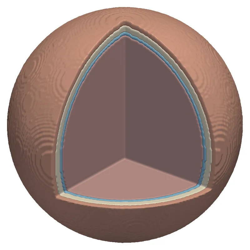
Electrosurgical needle in gel, surrounded by nested temperature-rise surfaces
Electrosurgery: heating around a needle in gel, from the same paper.
Founders

Built by the people who wrote the solvers

The founders develop the EMVIE solvers and carry out every study themselves, from model to report. Select a founder to read the full bio.

Contact

Bring us the exposure question you need answered.

A short description of the device, frequency and standard is enough for a first reply with a proposed scope and a fixed price. A non-disclosure agreement can be in place before you send any files.

info@corefieldbiophysics.com
Write to us
  • Medical device and implant makers
  • MRI coil and system developers
  • Wireless device makers and test laboratories
  • Neurostimulation developers and research groups
  • Teams that need an independent check of a simulation

Reza Gholami, PhD

Co-founder · Corefield Biophysics

Reza Gholami, PhD, builds electromagnetic solvers that make large, realistic problems computable, and is a research scientist at the École polytechnique fédérale de Lausanne (EPFL). Since 2026, in EPFL's Nanophotonics and Metrology Laboratory, Reza has led the numerical modelling of room-temperature terahertz quantum sensors for RythmiQs, a Swiss BRIDGE consortium, and developed fast solvers and adjoint-based inverse design for very large metasurfaces and metalenses. From 2025 to 2026, as a senior researcher at KU Leuven and EnergyVille, Reza developed finite-element harmonic-balance solvers with model order reduction for electric machines, a high-order hybrid FEM–BEM solver, and a biomedical electromagnetic solver for dosimetry in realistic human-body models.

From 2021 to 2025, Reza was a senior research and development engineer at Siemens Digital Industries Software (Siemens EDA) and a core developer of the HyperLynx 3D full-wave solver: layered-medium integral-equation methods and multilayer Green's functions for printed circuit boards and semiconductor packages, signal- and power-integrity and EMI/EMC analysis, and the solver's performance and robustness in production. Before that, as a postdoctoral fellow at the University of Toronto from 2019 to 2021, in collaboration with Thales Alenia Space, Reza developed fast integral-equation solvers for very large metasurfaces, reflectarrays and planar phased arrays for satellite communication payloads.

Reza holds a PhD in electrical and computer engineering from the University of Manitoba (2019), with work on direct and iterative integral-equation solvers for 3D problems with millions of unknowns, applied to the radar cross-section of full-scale aircraft, microwave scattering from sea ice and bio-electromagnetic studies on large human-body models. Reza also holds an MSc (2014) and a BSc (2011) in electrical and computer engineering from Babol Noshirvani University of Technology, and received a TICRA–EurAAP grant at the 14th European Conference on Antennas and Propagation (EuCAP).

At Corefield Biophysics, Reza co-develops the EMVIE solvers and their verification, and leads the research on 7 T transmit-array safety and on implant heating in MRI.

Core expertise

Nastaran Hendijani, PhD

Co-founder · Corefield Biophysics

Nastaran Hendijani, PhD, builds electromagnetic solvers and is a researcher at the University of Colorado Denver. As a senior research and development engineer at Ansys (part of Synopsys) from 2024, Nastaran worked on the core of Ansys Maxwell: its electrostatic, DC, AC and transient electric solvers and its frequency-domain and transient magnetic A-Phi solvers, adding new features to the finite-element A-Phi formulation and resolving complex solver issues reported by customers.

From 2015 to 2024, Nastaran was a research associate at the University of Colorado Denver, developing Magstrom, an electromagnetic simulation code funded by the U.S. Office of Naval Research: layered-media formulations, magnetostatics with permanent magnets, a broadband Huygens source model, a thin-layer magnetostatic volume integral equation, and augmented surface integral equations that stay accurate from very low to high frequencies.

Nastaran holds a PhD in electrical engineering from the University of Kentucky (2015), with a dissertation on the constrained locally corrected Nyström method, and an MS from Virginia Tech (2012), where the thesis work used radio-frequency identification to estimate the size of a stent implanted in an artery. The PhD work was a top-10 student paper finalist at ACES 2015.

Selected publications